ABAP
SAP- ABAP -Course Contents
Introduction
·
ERP
Overview
·
Business
Process in Enterprise
·
Various
ERP Packages
·
About
SAP
·
Features
and advantages of SAP
·
Technical
Features of SAP
Architecture of
R/3 System
·
Client/Server
Architecture
·
Two-tier
Vs Three tier Environments
·
Multi-tier
Architecture
·
Login
& Logoff Procedure
·
Navigation
·
Introduction
to SAP screen environment
Components of
ABAP Dictionary
·
Database
Tables
·
Data
Elements
·
Domains
·
Structures
·
Views:
Database View, Projections View,
·
Help
View, Maintenance View
·
Table
Types
·
Type
Groups
·
Search
Help: Elementary And Collective
·
Lock
Objects
ABAP
Programming
·
Introduction
to ABAP Editor
·
ABAP
Programming Features
·
Keywords
·
Data
Types and Data Objects
·
Operators
·
String
Handling
·
Conditional
Statements and Looping
·
Structures
·
Field
Symbols
·
ABAP
Development Workbench
·
Package
Builder
ABAP Database
Access
·
Open
SQL
·
Definition
& Creation of Internal Tables
·
Different
Internal Table Types
·
Different
Operations on Internal Tables
·
Control
Level Processing
·
Events
and Joins
Modularization
Techniques
·
Includes
·
Subroutines: Types, Pass by value, pass
·
by reference, pass by value and
·
reference
·
Function Modules, Exception Handling
Open SQL and
Additional Topics
·
Different Select Statements
·
Different Write Formats
·
Message Class
·
Selection Screen Designing
·
Inter programming Communication
List Generation
Techniques
·
List
Requirement & Introduction
·
Classical
List
·
Interactive
List
·
Abap
List Viewer
·
Logical
Database
Performance
Analysis
·
Reporting Standards
·
Extended Program Check
·
Debugger
·
Runtime Analysis
·
SQL Trace
·
Code Inspector
·
Advisable Select Statements
·
Performance Factors on Database
Tables and
Internal Tables
The Workbench
Organizer Transport System
·
Change Request Version Management
·
Releasing Tasks and Releasing Request
·
Transport
Dialog
Programming
·
Introduction
·
Screen Painter
·
Menu Painter
·
Table Control
·
Tab strip Control
·
Field Validation
·
Calling Screen Sequence
·
Changing Screen Attributes Dynamically
Data Migration
Techniques
·
Requirement
·
Direct Input Method
·
Background Processing
·
Conversion
·
Interface Programming Using BDC Call
·
Transaction and Session Method
·
Recording Method
·
Data Sets (Application Server File
·
Handling)
·
Legacy System Migration Workbench
·
(LSMW)
Smart Forms
·
Designing Custom Smart forms
·
Form Painter
·
Table Painter
·
Field List
·
Style Builder
·
Text Modules
·
Print Program
·
Overview of Interactive Forms by
·
Adobe
Object Oriented
ABAP
·
Introduction
·
Keywords
·
Class Builder
·
Objects
·
Local and Global Class Creation
·
Object Handling
·
Methods
·
Abstraction, Encapsulation
·
Inheritance, Polymorphism
·
Event Handling
·
Interface
Enhancements
·
Requirements
·
SMOD / CMOD
·
Function Exit
·
Menu Exit
·
Screen Exit
·
Text Enhancement
·
Table Enhancement
Business Add INS
·
Introduction to BAdIs
·
Difference between Customer Exists and
·
BAdIs
·
Implementation of BAdIs
·
Function Implementation
·
Screen Implementation
·
Menu Implementation
·
Definition of new BadIs
CROSS
APPLICATIONS
Introduction to
Distributed Database
Environment
·
Introduction to Cross Application
·
Architecture
·
Preparing RFC (Remote Function
·
Calling) Destinations
·
Develop and call Remote Functions
·
working with RFC function modules
IDOC Interface
·
Basics
·
Architecture
·
Segment Creation
·
Idoc Creation
·
Logical Messages
·
Processing Idoc
·
Monitoring
·
Documentation
·
Need in ALE, EDI and BAPI
·
Programming Idoc’s
·
Customer Modifications to the Idoc
·
Interface
·
Extending and Developing a Basic IDOC
·
Type
·
Programming in the IDoc Interface
·
Customizing the Interface for New or
·
Extended IDocs.
Remote Function
Call (RFC)
·
Introduction
·
Preparing RFC Destinations
·
Develop and call Remote Functions
·
Types of RFC
·
Synchronous RFC
·
Asynchronous RFC
·
Transactional RFC.
Application
Link Enabling (ALE)
·
Introduction,
·
Concepts of data and process
·
Distribution
·
Reasons for data and process
·
Distribution
·
ALE Concepts and Features
·
ALE Technology
·
ALE Components for Outbound Process
·
ALE Components for Inbound Process
·
Configuring ALE
·
Testing ALE
Electronic Data
Interchange (EDI)
·
Introduction,
·
EDI Standards,
·
History of EDI,
·
EDI Benefits
·
Configuring and Testing EDI in SAP
Business
Application Programming Interface
(BAPI)
·
Business Framework Architecture
·
Introduction to BOR,
·
Creating BAPI, R/3 to R/3, VB to R/3
·
Using Bapi, Java to R/3 using Bapi.
·
Reporting Using Bapi
·
Data Upload Using Bapi Structures
·
Working with BAPI Explorer
ABAP (Advanced Business Application Programming), originally Allgemeiner
Berichts-Aufbereitungs-Prozessor, German for “general report creation
processor” is a very high level programming language created by the German
software company SAP.

It is
currently positioned, alongside the more recently introduced Java, as the
language for programming SAP’s Web Application Server, part of its Net Weaver
platform for building business applications. Its syntax is somewhat similar to
COBOL.
ABAP
remains the language for creating programs for the client-server R/3 system,
which SAP first released in 1992. As computer hardware evolved through the
1990s, more and more of SAP’s applications and systems were written in ABAP. By
2001, all but the most basic functions were written in ABAP.
In 1999,
SAP released an object-oriented extension to ABAP called ABAP Objects, along
with R/3 release 4.6.
Introduction:
ABAP is
one of the many application-specific fourth-generation languages (4GLs) first
developed in the 1980s. It was originally the report language for SAP R/2, a
platform that enabled large corporations to build mainframe business
applications for materials management and financial and management accounting.
ABAP used
to be an abbreviation of Allgemeiner Berichtsaufbereitungsprozessor,
the German meaning of “generic report preparation processor”, but was later
renamed to Advanced Business Application Programming. ABAP was one of
the first languages to include the concept of Logical Databases (LDBs),
which provides a high level of abstraction from the basic database level.
The ABAP
programming language was originally used by developers to develop the SAP
R/3platform. It was also intended to be used by SAP customers to enhance SAP
applications – customers can develop custom reports and interfaces with
ABAP programming. The language is fairly easy to learn for programmers but it
is not a tool for direct use by non-programmers. Good programming skills,
including knowledge of relational database design and preferably also of
object-oriented concepts, are required to create ABAP programs.
ABAP
remains the language for creating programs for the client-server
R/3 system, which SAP first released in 1992. As computer hardware evolved
through the 1990s, more and more of SAP’s applications and systems were written
in ABAP. By 2001, all but the most basic functions were written in ABAP. In
1999, SAP released an object-oriented extension to ABAP called ABAP Objects,
along with R/3 release 4.6.

1.
History of ABAP
2. SAP R/3 Architecture and ABAP


3. ABAP Repository


4. ABAP Workbench


5. ABAP Workbench Tool

First find the SAP
icon on the desktop.


1.
History of ABAP
ABAP is a proprietary programming language of SAP and
ABAP stands for “Advanced Business Application Programming”.
Originally, known as Allgemeiner
Berichts-Aufbereitungs-Prozessor, German for general report creation processor
ABAP is a 4th Generation Programming
Language and was first developed in 1980s. By 1990s most of SAP’s application
software and systems were written in ABAP. In 1999 ABAP was extended to include
Object Oriented Programming. SAP’s most recent development is on ABAP as well
as JAVA platform.
Attributes and Prerequisites:
•
The language is fairly easy to learn for programmers
but it is not easy for use by nonprogrammers.
•
Knowledge of relational database design and preferably
also of object-oriented concepts is necessary to create ABAP programs.
•
The ABAP programming language allows SAP customers to
enhance SAP application programs – customers can develop custom reports and
interfaces with ABAP programming.
•
SAP ABAP programs all are stored in the SAP database
and not in form of separate external files like other program files eg Java,
c++, etc.
RDBMS
A relational database management system (RDBMS) is a
database management system (DBMS) that is based on the relational model as
introduced by E. F. Codd. Most popular databases currently in use are based on
the relational database model.
A short definition of an RDBMS is: a DBMS in which
data is stored in tables and the relationships among the data are also stored
in tables. The data can be accessed or reassembled in many different ways
without having to change the table forms.
A relational database is a database that conforms to
relational model theory. The software used in a relational database is called a
relational database management system (RDBMS). Colloquial use of the term
"relational database" may refer to the RDBMS software, or the
relational database itself. A relational database is the predominant choice in
storing data, over other models like the hierarchical database model or the
network model.
A relation is usually described as a table, which is
organized into rows and columns. All the data referenced by an attribute are in
the same domain and conform to the same constraints.
2. SAP R/3 Architecture and ABAP
SAP R/3 is based on Client Server Architecture and
the model is based on three-tier hierarchy.
The
presentation layer - User Interface (users interact with
the system with help of SAP
GUI or
through web-GUI)
The Application layer - All the programs related to business applications written in
ABAP are executed here.
The
Database layer - Data is stored
in this layer in a RDBMS.
Interaction between the different layers and ABAP:
The interaction between the user and the ABAP programs
which are executed in the Application layer is the main goal of this step by
step. ABAP programs are processed or executed in the application server. The
design of user interaction with the database is carried out via the ABAP
programs.
User accesses the application programs through the
SAP GUI which is installed on the presentation server.
•
User action like clicking on or
key, the control is passed from the presentation server to the
application server.
•
In the application Server, the ABAP program is
processed based on the user action and if needed further dialog is triggered
with the user by passing the control to the Presentation server, else if the
application needs access to the “data” to either retrieve data or store date,
the control of the program is passed to the Database Server.
•
On retrieving the data or saving the data, the Database
passes the control to the Application server and then the ABAP program passes
the information to the user when control is transferred back to the
Presentation Server.
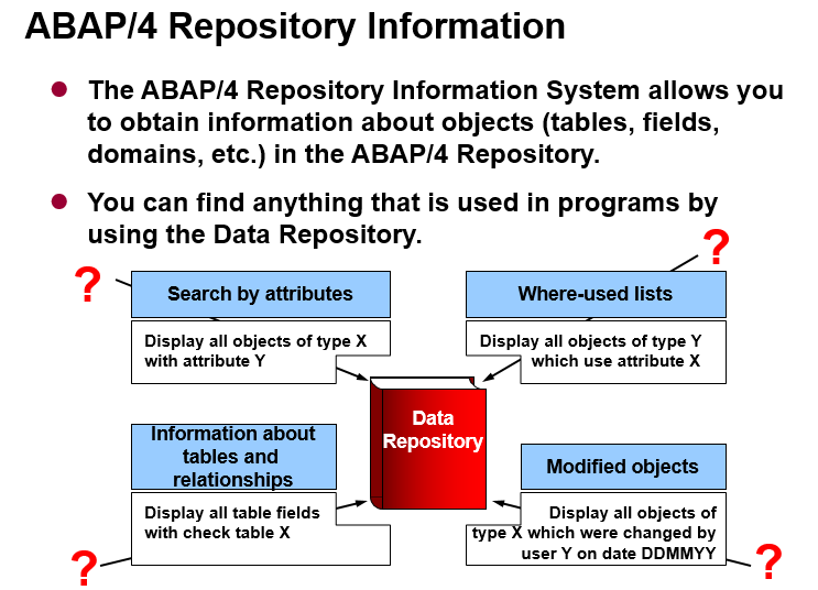
3. ABAP Repository
The Repository contains all of the development
objects of the system. The Repository is used to store both objects – defined
by SAP as well as objects defined by customers.
Attributes of Repository objects:
•
The Repository is in the SAP system’s central database
•
The Repository objects are client independent – means that Repository objects can be accessed
from any client.
•
The Repository is sub-divided depending on application
components called subobjects.
•
A Repository Object is always assigned to a development
class called package from ECC.
To reach the Repository the menu path is as follows:
Menu Path:
SAP Easy Access →
Tools →
ABAP Workbench → Overview → Information System
TCode = SE84
The repository structure can be viewed by selecting a
component from the tree structure.
Double click on a object type you want information on,
a selection screen will be displayed to help facilitate the search.
4. ABAP Workbench
The ABAP Workbench includes all the tools required
for maintaining Repository Objects for development of application
programs.
The various tools are:
•
ABAP Editor
•
Data Dictionary
•
Menu Painter
•
Screen Painter
•
Function Builder
•
Debugger
•
Object Navigator
Each of the tools can be called explicitly and then a
Repository object loaded for processing.
Object Navigator is a single point tool to access all
the workbench objects.
To reach the ABAP
Workbench for development, the menu path is as follows:
Menu Path:
SAP
Easy Access → Tools → ABAP Workbench →
Development
All the development objects, ABAP Editor, Data
Dictionary, Function Builder, etc required for the maintenance of the
Repository are under this menu option.
One can go to any application in the system by
navigating through the menu path or by entering the transaction codes for the
application in the “command” field.
Transaction Codes:
Each function / application in the SAP system is
assigned a transaction code. A transaction code consists of letters, numbers or
both. You enter transaction code in the command field which will take you to
the SAP application faster as against navigating via menu path.

•
A transaction code can be up to 20 characters long
•
A transaction code should begin with a letter
•
Enter the transaction code in the “Command Field” and
choose <>
Command Field:
The command field is on the standard tool bar and
you can either hide the command field or display it by choosing the arrow to
the left of the “SAVE” icon.
To display the
transaction codes for the applications, there are 2 ways:
1.
If you are in an application, and want to know the
transaction code for the same, then from the menu bar, choose System ->
Status and in the system status dialog box, the transaction code for the
current application will be displayed.
In the status, you will get the transaction code
1.
If you need to display transaction code against all
application while navigating through the menu path.
Menu Path:
SAP Easy Access → Menu Bar →
Extras →
Settings
Check “Display Technical Names” in settings. Click on
<< Enter >>
5. ABAP Workbench Tool
The tools in the Workbench are integrated. When you
are working on a program, the ABAP Editor will also recognize objects created
using other tools. This integration allows you to double-click an object, the
Workbench automatically launches the tool that was used to create the object.
SAP’s Object Navigator helps organize your
application development in this integrated environment. It provides a context
that makes it easier for you to trace the relationships between objects in a
program. Rather than working with tools and packages separately, you work with
objects and allow the Workbench to launch the appropriate tool for an object.
a. Development Objects and Packages
When you work with the Workbench, you work with
development objects and packages.
Development objects are the individual parts of an
ABAP application like reports, transactions, and function modules. Program
components such as events, screens, menus, and function modules are also
development objects. Objects that programs can share are development objects as
well. These shareable objects include database fields, field definitions, and
program messages.
A package is a container for objects that logically
belong together; for example, all of the objects in an application. A package
is also a type of development object. An example of a package might be General
Ledger Accounting.
When you create a new object or change an existing
object, the system asks you to assign the object to a package.
b. Storing Development Objects
The SAP system stores development objects in the
Repository, which is a part of the database.
When you complete work on a development object like
a program, screen, or menu, you generate a runtime version of the object. This
runtime version is stored, along with the object, in the Repository. An
application consists of several runtime objects that are processed by the work
processes in the SAP System.
In a standard SAP installation, development and live
operation take place in separate systems. New applications are created in the
development system and transported to the production system. Daily work takes
place in the production system which uses runtime versions created in the
development system.
The division between production and development
systems is recommended because changes to an existing ABAP application take
immediate effect. To prevent disturbances in daily work flow in the production
system, all developments are carried out in development systems designed
especially for this purpose.
c. The Transport Organizer
The Transport Organizer is used to move applications
from the development system to the production system. The Workbench Organizer
also provides version control and tracking.
(** Refer to chapter-14 for details)
Naming
Standards (Nomenclature):
•
Any custom developed objects name should start with a
letter “Z” or “Y”.
•
SAP reserves the letters from “A” to “X” for naming their
own objects.
•
The rest of the naming convention will be
client/organization specific.
ABAP
Programming Syntax:
•
ABAP Programs are made up of individual statement.
•
Each statement begins with a “Keyword”.
•
Each statement ends with a “period”.
•
Words can be separated by at least one space.
•
Statements can occupy more than one line • Statements can be indented for readability purpose.
•
ABAP Programs are interpreted, not compiled.
•
The first time the program is executed, the system
automatically generates a runtime object.
6. ABAP Keys:
There are 2 types of Keys in SAP ABAP:
1.
Developer’s Key
2.
Access Key
a. ABAP Developer’s Key:
A Developer key –
Allows a user to develop custom objects (can be new programs, database tables, functions, or
any other work bench object).
A SAP Developer requires 2 things to work on custom
development object using ABAP Workbench and they are:
1.
Authorization to work with ABAP Workbench object
2.
Developer Access key
Above both, are assigned to the SAP user depending
on their role, by the BASIS Team usually.
•
Authorizations to work with ABAP Development objects,
is provided by the BASIS team in the Developer’s profile.
•
The “Developer Key” is a 20 digit key associated with a
user-name and is unique and assigned by BASIS team.
•
The Developer key for the User-Id is requested in the
SAP Service Market Place by the BASIS team,
Without the Developer Key, if a Developer tries to
work on any custom workbench object, they will receive a message to register
the developer and validate it by entering the Developer Key as displayed
below:
Click on <>, on entering a
valid key, permission will be granted for working with the Workbench
Objects.
The Developer Key is entered only one time and it
registers the user-name for Development roles.
Double click on the SAP icon.
On the logon pad select the system you want to login to and press log on
button.
Enter Client, User, password and press enter.
This is
SAP easy access screen. All the tools required by ABAP developer is under the
node Tools.
Let us
write a “Hello SAP ABAP” program.
Navigate
to ABAP editor under Tools node in SAP easy access.

Double
click on “ABAP Editor” to open the editor. ABAP editor can also be opened by
entering t-code SE38 in the command field.


This is
the ABAP editor’s initial screen. Enter the name of the program you want to
create and press create. All the customer programs must begin with “Y” or “Z”.
In the
next popup screen(Program attributes) enter the title for your program,
select Executable program as type and press save.
Press Local Object to store the program in the temporary folder
This is
the screen where you can write the ABAP code.
Write the
code. Press save, then syntax check (Ctrl + F2).
If there
are any syntax errors, it will be displayed at the bottom of the screen as
shown above. Correct the errors and again check the syntax.
Successful
syntax check message will be displayed in the status bar. Then activate (Ctrl +
F3) the program.
In the
following screen select your program and press continue. Then run (F8) the
program.
The output
will be displayed as shown above.


*******************************SQL***********************


INDEX .


Menu bar:
The Menu bar is the top line of any dialog window in
the SAP system.
Standard toolbar:
Standard functions that are
available in displayed in this toolbar. The applications like save, top of
page, end of page, page up, page down, print, etc.
Title bar:
Displays the name of the application/business
process you are currently in.
Application toolbar:
Application specific menu options are available on
this toolbar.
Command Field:
To start a business application
without having to navigate through the menu transaction codes are assigned to
the business processes. Transaction codes are entered in the command field to
directly start the application.
b.
Standard
Toolbar Icons:
e. Login Off:
It is a good practice to log off
from the SAP system when you finish your work. There are several ways of login
off from the system:
•
From Menu, select system -> log off
•
Close the open sessions and the last session will log
you off
•
Enter /nex in the command field
Before the system logs you out, a
dialog box is displayed to confirm you want to log off from the system, except
for the option /nex in the command field.
IF –
Branching Conditionally
IF statement – The code between IF and ENDIF is executed only if the condition is true.
IF statement – The code between IF and ENDIF is executed only if the condition is true.
DATA: a
TYPE i VALUE 10. " We can assign a
value in the declaration
IF a >
5.
WRITE:/ 'Condition True'.
ENDIF.
output:
IF-ELSE
statement – The code between IF and ELSE is executed
if the condition is true, the code between ELSE andENDIF is
executed if the condition is False.
DATA: a
TYPE i VALUE 1.
IF a >
5.
WRITE:/ 'Condition True'.
ELSE.
WRITE:/ 'Condition False'.
ENDIF.
Output
IF-ELSEIF
statement – Used to check multiple conditions.
DATA: a
TYPE i VALUE 2.
IF a >
5.
WRITE:/ a, 'Greater Than', 5.
ELSEIF a
> 4.
WRITE:/ a, 'Greater Than', 4.
ELSEIF a
> 3.
WRITE:/ a, 'Greater Than', 3.
ELSE.
WRITE:/ a, 'Less Than', 3.
ENDIF.
Output
CASE-ENDCASE –
Branching based on the content of the variable.
DATA: a
TYPE i VALUE 4.
CASE a.
WHEN 3.
WRITE:/ a, 'Equals', 3.
WHEN 4.
WRITE:/ a, 'Equals', 4.
WHEN OTHERS.
WRITE:/ 'Not Found'.
ENDCASE.
Output:
When no
condition is met, OTHERS will be executed. OTHERS is not
mandatory.
*
DO – ENDDO
– Unconditional Loop
DO can be used to execute a certain lines of codes specific number of times.
DO can be used to execute a certain lines of codes specific number of times.
DO 5
TIMES.
WRITE sy-index. " SY-INDEX (system variable) - Current
loop pass
ENDDO.
Output
WHILE
ENDWHILE – Conditional Loop
WHILE can
be used to execute a certain lines of codes as long as the condition is true.
WHILE
sy-index < 3.
WRITE sy-index.
ENDWHILE.
Output
CONTINUE –
Terminate a loop pass unconditionally.
After
continue the control directly goes to the end statement of the current loop
pass ignoring the remaining statements in the current loop pass, starts the
next loop pass.
DO 5
TIMES.
IF sy-index = 2.
CONTINUE.
ENDIF.
WRITE sy-index.
ENDDO.
Output
CHECK –
Terminate a loop pass conditionally.
If the
condition is false, the control directly goes to the end statement of the
current loop pass ignoring the remaining statements in the current loop pass,
starts the next loop pass.
DO 5
TIMES.
CHECK sy-index < 3.
WRITE sy-index.
ENDDO.
Output
EXIT –
Terminate an entire loop pass unconditionally.
After EXIT
statement the control goes to the next statement after the end of loop
statement.
DO 10
TIMES.
IF sy-index = 2.
EXIT.
ENDIF.
WRITE sy-index.
ENDDO.
Output
*******************************SQL***********************
DATA:
gwa_employee TYPE zemployee.
WRITE:/1
'Emp ID' color 5,9 'Name' color 5,17 'Place' color 5,
27 'Phone' color 5,39 'Dept' color 5.
SELECT *
FROM zemployee INTO gwa_employee.
WRITE:/1 gwa_employee-id,9 gwa_employee-name,
17 gwa_employee-place,27
gwa_employee-phone,
39 gwa_employee-dept_id.
ENDSELECT.
In the
above code,
GWA_EMPLOYEE
is the work area to hold one record of table ZEMPLOYEE at a time.
SELECT
* specifies all the rows and columns are read from the database.
SELECT –
ENDSELECT works in a loop, so the code between SELECT and ENDSELECT will be
executed for each record found in the database table.
WRITE
statements are used to output the values in the list.
If the
SELECT statement returns any record then the value of the system variable
SY-SUBRC is set to zero else a non zero value will be set.
After the
SELECT statement is executed, the value of the system variable SY-DBCNT
contains the number of records read from the database. The value of SY-DBCNT is
zero if no records are read from the database.
Table
ZEMPLOYEE Entries
Report
Output:
Let us
write a program to read only the employees with department ID 2.
DATA:
gwa_employee TYPE zemployee.
WRITE:/1
'Emp ID' COLOR 5,9 'Name' COLOR 5,17 'Place' COLOR 5,
27 'Phone' COLOR 5,39 'Dept' COLOR 5.
SELECT *
FROM zemployee INTO gwa_employee
WHERE dept_id = 2.
WRITE:/1 gwa_employee-id,9 gwa_employee-name,
17 gwa_employee-place,27
gwa_employee-phone,
39 gwa_employee-dept_id.
ENDSELECT.
Report Output:
What if we
want to select only certain columns from the database table instead of all the
columns? Then we need to specify the field list(field names) in the SELECT
statement instead of specifying ‘*’.
SELECT id
phone dept_id FROM zemployee INTO CORRESPONDING FIELDS OF
gwa_employee
WHERE dept_id = 2.
WRITE:/1 gwa_employee-id,9 gwa_employee-name,
17 gwa_employee-place,27
gwa_employee-phone,
39 gwa_employee-dept_id.
ENDSELECT.
Report
Output:
Only
columns ID, PHONE and DEPT_ID were read from the database.
To select
a single record from the database use SELECT SINGLE instead of SELECT
statement. SELECT SINGLE picks the first record found in the database that
satisfies the condition in WHERE clause. SELECT SINGLE does not work in loop,
so no ENDSELECT is required.
SELECT
SINGLE * FROM zemployee INTO gwa_employee
WHERE dept_id = 2.
WRITE:/1
gwa_employee-id,9 gwa_employee-name,
17 gwa_employee-place,27
gwa_employee-phone,
39 gwa_employee-dept_id.
Report
Output:
INSERT is
the open SQL statement to add values to the database table. First declare a
work area as the line structure of database table and populate the work area
with the desired values. Then add the values in the work area to the database
table using INSERT statement.
The syntax
for the INSERT statement is as follows.
INSERT
FROM
or
INSERT
INTO VALUES
If the
database table does not already contain a line with the same primary key as
specified in the work area, the operation is completed successfully and
SY-SUBRC is set to 0. Otherwise, the line is not inserted, and SY-SUBRC is set
to 4.
DATA:
gwa_employee TYPE zemployee.
gwa_employee-id = 6.
gwa_employee-name = 'MARY'.
gwa_employee-place = 'FRANKFURT'.
gwa_employee-phone = '7897897890'.
gwa_employee-dept_id
= 5.
INSERT
zemployee FROM gwa_employee.
EMPLOYEE
table entries before INSERT
EMPLOYEE
table entries after INSERT
UPDATE is
the open SQL statement to change the values in the database table. First
declare a work area as the line structure of database table and populate the
work area with the desired values for a specific key in the database table.
Then update the values for the specified key in the database table using UPDATE
statement.
The syntax
for the UPDATE statement is as follows.
UPDATE
FROM
If the
database table contains a line with the same primary key as specified in the
work area, the operation is completed successfully and SY-SUBRC is set to 0.
Otherwise, the line is not inserted, and SY-SUBRC is set to 4.
DATA:
gwa_employee TYPE zemployee.
gwa_employee-id = 6.
gwa_employee-name = 'JOSEPH'.
gwa_employee-place = 'FRANKFURT'.
gwa_employee-phone = '7897897890'.
gwa_employee-dept_id
= 5.
UPDATE
zemployee FROM gwa_employee.
EMPLOYEE
table entries before UPDATE
EMPLOYEE
table entries after UPDATE
We can
also change certain columns in the database table using the following syntax
UPDATE
SET … [WHERE ].
The WHERE
clause determines the lines that are changed. If we do not specify a WHERE
clause, all lines will be changed.
UPDATE
zemployee SET place = 'MUMBAI' WHERE dept_id = 2.
EMPLOYEE
table entries after UPDATE
DELETE is
the open SQL statement to delete entries from database table. First declare a
work area as the line structure of database table and populate the work area
with the specific key that we want to delete from the database table.
Then delete the entries from the database table using DELETE statement.
The syntax
for the DELETE statement is as follows.
DELETE
FROM
If the
database table contains a line with the same primary key as specified in the
work area, the operation is completed successfully and SY-SUBRC is set to 0.
Otherwise, the line is not deleted, and SY-SUBRC is set to 4.
DATA:
gwa_employee TYPE zemployee.
gwa_employee-id = 6.
gwa_employee-name = 'JOSEPH'.
gwa_employee-place = 'FRANKFURT'.
gwa_employee-phone = '7897897890'.
gwa_employee-dept_id
= 5.
DELETE
zemployee FROM gwa_employee.
EMPLOYEE
table entries before DELETE
EMPLOYEE
table entries after DELETE
We can
also multiple lines from the table using the WHERE clause in the DELETE statement.
DELETE
FROM WHERE
DELETE
FROM zemployee WHERE dept_id = 2.
EMPLOYEE
table entries after DELETE
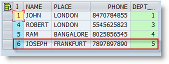
MODIFY is
the open SQL statement to insert or change entries in the database table. If
the database table contains no line with the same primary key as the line to be
inserted, MODIFY works like INSERT, that is, the line is added. If the database
already contains a line with the same primary key as the line to be inserted,
MODIFY works like UPDATE, that is, the line is changed.
The syntax
for the MODIFY statement is as follows.
MODIFY
FROM
If the
database table does not already contain a line with the same primary key as
specified in the work area, a new line is inserted. If the database table does
already contain a line with the same primary key as specified in the work area,
the existing line is overwritten. SY-SUBRC is always set to 0.
DATA:
gwa_employee TYPE zemployee.
gwa_employee-id = 6.
gwa_employee-name = 'JOSEPH'.
gwa_employee-place = 'FRANKFURT'.
gwa_employee-phone = '7897897890'.
gwa_employee-dept_id
= 5.
MODIFY
zemployee FROM gwa_employee.
ZEMPLOYEE
table entries before MODIFY
ZEMPLOYEE
table entries after MODIFY
Since
there was no entry with the key 6, a new entry was added to the table.
DATA:
gwa_employee TYPE zemployee.
gwa_employee-id = 6.
gwa_employee-name = 'JOHNNY'.
gwa_employee-place = 'LONDON'.
gwa_employee-phone = '7897897890'.
gwa_employee-dept_id
= 3.
MODIFY
zemployee FROM gwa_employee.
Since
there was an entry with the key 6, the values in the existing record were
modified.
**************************JOINS***********************
An
Internal table is a temporary table gets created in the memory of application
server during program execution and gets destroyed once the program ends. It is
used to hold data temporarily or manipulate the data. It contains one or more
rows with same structure.
An
internal table can be defined using the keyword TABLE OF in the DATA statement.
Internal table can be defined by the following ways.
TYPES:
BEGIN OF ty_student,
id(5)
TYPE n,
name(10) TYPE c,
END OF ty_student.
DATA:
gwa_student TYPE ty_student.
"Referring
to local data type
DATA: it1
TYPE TABLE OF ty_student.
"Referring
to local data object
DATA: it2
LIKE TABLE OF gwa_student.
"Referring
to data type in ABAP dictionary
DATA: it3
TYPE TABLE OF mara.
Use the
APPEND statement to add data to internal table. First define the work area i.e.
define a field string with a structure similar to row of the internal table.
Then place the data in the work area and use the APPEND statement to add the
data from work area to internal table.
*--------------------------------------------------------------*
*Data
Types
*--------------------------------------------------------------*
TYPES:
BEGIN OF ty_student,
id(5)
TYPE n,
name(10) TYPE c,
END OF ty_student.
DATA: gwa_student TYPE ty_student.
*--------------------------------------------------------------*
*Data
Declaration
*--------------------------------------------------------------*
"Referring
to local data type
DATA: it
TYPE TABLE OF ty_student.
gwa_student-id = 1.
gwa_student-name = 'JOHN'.
APPEND
gwa_student TO it.
gwa_student-id = 2.
gwa_student-name = 'JIM'.
APPEND
gwa_student TO it.
gwa_student-id = 3.
gwa_student-name = 'JACK'.
APPEND
gwa_student TO it.
After the
last APPEND statement in the above program, internal table ‘IT’ has the
following 3 entries. But the internal table values are not persistent i.e. the
internal table and its values are discarded once the program ends.
ID
|
NAME
|
1
|
JOHN
|
2
|
JIM
|
3
|
JACK
|
Usually
internal tables are used to hold data from database tables temporarily for
displaying on the screen or further processing. To fill the internal table with
database values, use SELECT statement to read the records from the database one
by one, place it in the work area and then APPEND the values in the work area to
internal table.
DATA:
gwa_employee TYPE zemployee,
gt_employee TYPE TABLE OF zemployee.
SELECT *
FROM zemployee INTO gwa_employee.
APPEND gwa_employee TO gt_employee.
ENDSELECT.
After
ENDSELECT the internal table GT_EMPLOYEE contains all the records that are
present in table ZEMPLOYEE.
Using INTO
TABLE addition to SELECT statement we can also read multiple records directly
into the internal table directly. No work area used in this case. This select
statement will not work in loop, so no ENDSELECT is required.
SELECT *
FROM zemployee INTO TABLE gt_employee.
We can
insert one or more lines to ABAP internal tables using the INSERT statement. To
insert a single line, first place the values we want to insert in a work area
and use the INSERT statement to insert the values in the work area to internal
table.
Syntax to
insert a line to internal table
INSERT
INTO TABLE .
OR
INSERT
INTO INDEX .
The first
INSERT statement without INDEX addition will simply add the record to the end
of the internal table. But if we want to insert the line to specific location
i.e. if we want to insert it as second record then we need to specify 2 as the
index in the INSERT statement.
*--------------------------------------------------------------*
*Data
Types
*--------------------------------------------------------------*
TYPES:
BEGIN OF ty_student,
id(5)
TYPE n,
name(10) TYPE c,
END OF ty_student.
*--------------------------------------------------------------*
*Data
Declaration
*--------------------------------------------------------------*
DATA:
gwa_student TYPE ty_student.
DATA: it
TYPE TABLE OF ty_student.
gwa_student-id = 1.
gwa_student-name = 'JOHN'.
INSERT
gwa_student INTO TABLE it.
gwa_student-id = 2.
gwa_student-name = 'JIM'.
INSERT
gwa_student INTO TABLE it.
gwa_student-id = 3.
gwa_student-name = 'JACK'.
INSERT
gwa_student INTO TABLE it.
WRITE:/
'ID' COLOR 5,7 'Name' COLOR 5.
LOOP AT it
INTO gwa_student.
WRITE:/ gwa_student-id, gwa_student-name.
ENDLOOP.
SKIP.
WRITE:/
'After using Index addition' COLOR 4.
gwa_student-id = 4.
gwa_student-name = 'RAM'.
INSERT
gwa_student INTO it INDEX 2.
WRITE:/
'ID' COLOR 5,7 'Name' COLOR 5.
LOOP AT it
INTO gwa_student.
WRITE:/ gwa_student-id, gwa_student-name.
ENDLOOP.
Output:
We can
also insert multiple lines to an internal table with a single INSERT statement
i.e. we can insert the lines of one internal table to another internal table.
Syntax to
insert multiple lines to internal table
INSERT
LINES OF [FROM ] [TO ] INTO TABLE
.
OR
INSERT
LINES OF [FROM ] [TO ] INTO
*--------------------------------------------------------------*
*Data
Types
*--------------------------------------------------------------*
TYPES:
BEGIN OF ty_student,
id(5)
TYPE n,
name(10) TYPE c,
END OF ty_student.
*--------------------------------------------------------------*
*Data
Declaration
*--------------------------------------------------------------*
DATA:
gwa_student TYPE ty_student.
DATA:
it TYPE TABLE OF ty_student,
it2 TYPE TABLE OF ty_student,
it3 TYPE TABLE OF ty_student,
it4 TYPE TABLE OF ty_student.
gwa_student-id = 1.
gwa_student-name = 'JOHN'.
INSERT
gwa_student INTO TABLE it.
gwa_student-id = 2.
gwa_student-name = 'JIM'.
INSERT
gwa_student INTO TABLE it.
gwa_student-id = 3.
gwa_student-name = 'JACK'.
INSERT
gwa_student INTO TABLE it.
gwa_student-id = 4.
gwa_student-name = 'ROB'.
INSERT
gwa_student INTO TABLE it.
WRITE:/
'Inserting all the lines of IT to IT2' COLOR 4.
INSERT
LINES OF it INTO TABLE it2.
WRITE:/
'Display values of IT2' COLOR 1.
WRITE:/
'ID' COLOR 5,7 'Name' COLOR 5.
LOOP AT
it2 INTO gwa_student.
WRITE:/ gwa_student-id, gwa_student-name.
ENDLOOP.
SKIP.
WRITE:/
'Inserting only lines 2 & 3 of IT to IT3' COLOR 4.
INSERT
LINES OF it FROM 2 TO 3 INTO TABLE it3.
WRITE:/
'Display values of IT3' COLOR 1.
WRITE:/
'ID' COLOR 5,7 'Name' COLOR 5.
LOOP AT
it3 INTO gwa_student.
WRITE:/ gwa_student-id, gwa_student-name.
ENDLOOP.
gwa_student-id = 1.
gwa_student-name = 'RAM'.
INSERT
gwa_student INTO TABLE it4.
gwa_student-id = 4.
gwa_student-name = 'RAJ'.
INSERT
gwa_student INTO TABLE it4.
SKIP.
WRITE:/
'Inserting only lines 2 & 3 of IT to IT4 at 2' COLOR 4.
INSERT
LINES OF it FROM 2 TO 3 INTO it4 INDEX 2.
WRITE:/
'Display values of it4' COLOR 1.
WRITE:/
'ID' COLOR 5,7 'Name' COLOR 5.
LOOP AT
it4 INTO gwa_student.
WRITE:/ gwa_student-id, gwa_student-name.
ENDLOOP.
The last
INSERT statement in the above program inserts the 2nd and 3rd line from IT at
index 2 in IT4, so the new lines inserted becomes the 2nd and 3rd line in IT4.
Output:
MODIFY is
the statement to change single or multiple lines in an internal table. Use the INDEX addition to change
a single line. If we use the INDEX addition and the operation is successful,
SY-SUBRC will be set to zero and the contents of the work area overwrites the
contents of the line with the corresponding index.
Instead of
changing all the values of a row we can specify the fields we want to change by
specifying the fieldnames in the TRANSPORTING addition.
MODIFY
FROM [INDEX ]
[TRANSPORTING
... ].
We can
also use the above MODIFY statement without INDEX addition inside LOOP. Inside
LOOP if we do not specify the INDEX, then the current loop line will be
modified.
We can use
the WHERE clause to change single or multiple lines. All the lines that meet
the logical condition will be processed. If at least one line is changed, the
system sets SY-SUBRC to 0, otherwise to 4.
MODIFY
FROM
TRANSPORTING
... WHERE .
*--------------------------------------------------------------*
*Data
Types
*--------------------------------------------------------------*
TYPES:
BEGIN OF ty_student,
id(5)
TYPE n,
name(10)
TYPE c,
place(10) TYPE c,
age
TYPE i,
END OF ty_student.
*--------------------------------------------------------------*
*Data
Declaration
*--------------------------------------------------------------*
DATA:
gwa_student TYPE ty_student.
DATA:
it TYPE TABLE OF ty_student.
gwa_student-id = 1.
gwa_student-name = 'JOHN'.
gwa_student-place = 'London'.
gwa_student-age = 20.
INSERT
gwa_student INTO TABLE it.
gwa_student-id = 2.
gwa_student-name = 'JIM'.
gwa_student-place = 'New York'.
gwa_student-age = 21.
INSERT
gwa_student INTO TABLE it.
gwa_student-id = 3.
gwa_student-name = 'JACK'.
gwa_student-place = 'Bangalore'.
gwa_student-age = 20.
INSERT
gwa_student INTO TABLE it.
gwa_student-id = 4.
gwa_student-name = 'ROB'.
gwa_student-place = 'Bangalore'.
gwa_student-age = 22.
INSERT
gwa_student INTO TABLE it.
WRITE:/
'Values in IT before MODIFY' COLOR 4.
WRITE:/
'ID' COLOR 5,7 'Name' COLOR 5, 18 'Place' COLOR 5,
37 'Age' COLOR 5.
LOOP AT it
INTO gwa_student.
WRITE:/ gwa_student-id, gwa_student-name,
gwa_student-place,
gwa_student-age.
ENDLOOP.
SKIP.
WRITE:/
'Values in IT after MODIFY' COLOR 4.
gwa_student-id = 4.
gwa_student-name = 'ROB'.
gwa_student-place = 'Mumbai'.
gwa_student-age = 25.
*Change
all the columns of row 4 with work area values
MODIFY it
FROM gwa_student INDEX 4.
WRITE:/
'ID' COLOR 5,7 'Name' COLOR 5, 18 'Place' COLOR 5,
37 'Age' COLOR 5.
LOOP AT it
INTO gwa_student.
WRITE:/ gwa_student-id, gwa_student-name,
gwa_student-place,
gwa_student-age.
ENDLOOP.
SKIP.
WRITE:/
'Values in IT after Transporting addition' COLOR 4.
gwa_student-id = 9.
gwa_student-name = 'TOM'.
gwa_student-place = 'Bangalore'.
gwa_student-age = 30.
*Change
specific columns of row 4 with work area values by
*using
TRANSPORTING addition
MODIFY it
FROM gwa_student INDEX 4 TRANSPORTING place.
WRITE:/
'ID' COLOR 5,7 'Name' COLOR 5, 18 'Place' COLOR 5,
37 'Age' COLOR 5.
LOOP AT it
INTO gwa_student.
WRITE:/ gwa_student-id, gwa_student-name,
gwa_student-place,
gwa_student-age.
ENDLOOP.
SKIP.
WRITE:/
'Values in IT after MODIFY using WHERE Clause' COLOR 4.
gwa_student-place = 'Mumbai'.
*Change
multiple rows using WHERE clause
MODIFY it
FROM gwa_student TRANSPORTING place
WHERE place =
'Bangalore'.
WRITE:/
'ID' COLOR 5,7 'Name' COLOR 5, 18 'Place' COLOR 5,
37 'Age' COLOR 5.
LOOP AT it
INTO gwa_student.
WRITE:/ gwa_student-id, gwa_student-name,
gwa_student-place,
gwa_student-age.
ENDLOOP.
Output:
DELETE is
the statement to delete one or more lines from an ABAP Internal Table. Use the INDEX addition to delete
a single line. If we use the INDEX addition and the operation is successful,
SY-SUBRC will be set to zero, the line with the corresponding index in
the internal table will be deleted and the indexes of the subsequent lines will
be reduced by one.
DELETE
[INDEX ].
We can
also use the above DELETE statement without INDEX addition inside LOOP. Inside
LOOP if we do not specify the INDEX, then the current loop line will be
deleted.
We can use
the WHERE clause to delete single or multiple lines. All the lines that meet
the logical condition will be deleted. If at least one line is deleted, the
system sets SY-SUBRC to 0, otherwise to 4.
DELETE
[FROM ] [TO ] [WHERE
].
With WHERE
clause we can also specify the lines between certain indices that we want to
delete by specifying indexes in FROM and TO additions.
*--------------------------------------------------------------*
*Data
Types
*--------------------------------------------------------------*
TYPES:
BEGIN OF ty_student,
id(5)
TYPE n,
name(10)
TYPE c,
place(10) TYPE c,
age
TYPE i,
END OF ty_student.
*--------------------------------------------------------------*
*Data
Declaration
*--------------------------------------------------------------*
DATA:
gwa_student TYPE ty_student.
DATA:
it TYPE TABLE OF ty_student.
gwa_student-id = 1.
gwa_student-name = 'JOHN'.
gwa_student-place = 'London'.
gwa_student-age = 20.
INSERT
gwa_student INTO TABLE it.
gwa_student-id = 2.
gwa_student-name = 'JIM'.
gwa_student-place = 'New York'.
gwa_student-age = 21.
INSERT
gwa_student INTO TABLE it.
gwa_student-id = 3.
gwa_student-name = 'JACK'.
gwa_student-place = 'Bangalore'.
gwa_student-age = 20.
INSERT
gwa_student INTO TABLE it.
gwa_student-id = 4.
gwa_student-name = 'ROB'.
gwa_student-place = 'Bangalore'.
gwa_student-age = 22.
INSERT
gwa_student INTO TABLE it.
WRITE:/
'Values in IT before DELETE' COLOR 4.
WRITE:/
'ID' COLOR 5,7 'Name' COLOR 5, 18 'Place' COLOR 5,
37 'Age' COLOR 5.
LOOP AT it
INTO gwa_student.
WRITE:/ gwa_student-id, gwa_student-name,
gwa_student-place,
gwa_student-age.
ENDLOOP.
SKIP.
WRITE:/
'Values in IT after DELETE' COLOR 4.
*Delete
second line from IT
DELETE it
INDEX 2.
WRITE:/
'ID' COLOR 5,7 'Name' COLOR 5, 18 'Place' COLOR 5,
37 'Age' COLOR 5.
LOOP AT it
INTO gwa_student.
WRITE:/ gwa_student-id, gwa_student-name,
gwa_student-place,
gwa_student-age.
ENDLOOP.
SKIP.
WRITE:/
'Values in IT after DELETE using WHERE Clause' COLOR 4.
*Delete
entries from IT where place is Bangalore
DELETE it
WHERE place = 'Bangalore'.
WRITE:/
'ID' COLOR 5,7 'Name' COLOR 5, 18 'Place' COLOR 5,
37 'Age' COLOR 5.
LOOP AT it
INTO gwa_student.
WRITE:/ gwa_student-id, gwa_student-name,
gwa_student-place,
gwa_student-age.
ENDLOOP.
Output:
DESCRIBE
TABLE is the statement to get the attributes like number of lines, line width
of each row etc. of the internal table. DESCRIBE TABLE statement also
fills the system fields SY-TFILL (Current no. of lines in internal table),
SY-TLENG (line width of internal table) etc.
DESCRIBE
TABLE [LINES ].
SORT is
the statement to sort an ABAP internal table. We can specify the direction of
the sort using the additions ASCENDING and DESCENDING. The default is
ascending.
SORT
[ASCENDING|DESCENDING]
We can
also delete the adjacent duplicates from an internal table by using the
following statement.
DELETE
ADJACENT DUPLICATE ENTRIES FROM
[COMPARING
... |ALL FIELDS].
COMPARING
ALL FIELDS is the default. If we do not specify the COMPARING addition, then
the system compares all the fields of both the lines. If we specify fields in
the COMPARING clause, then the system compares only the fields specified after
COMPARING of both the lines. If at least one line is deleted, the system sets
SY-SUBRC to 0, otherwise to 4.
*--------------------------------------------------------------*
*Data Types
*--------------------------------------------------------------*
TYPES:
BEGIN OF ty_student,
id(5)
TYPE n,
name(10)
TYPE c,
place(10) TYPE c,
age
TYPE i,
END OF ty_student.
*--------------------------------------------------------------*
*Data
Declaration
*--------------------------------------------------------------*
DATA:
gwa_student TYPE ty_student.
DATA:
it TYPE TABLE OF ty_student.
DATA:
gv_lines TYPE i.
gwa_student-id = 1.
gwa_student-name = 'JOHN'.
gwa_student-place = 'London'.
gwa_student-age = 20.
APPEND
gwa_student TO it.
gwa_student-id = 2.
gwa_student-name = 'JIM'.
gwa_student-place = 'New York'.
gwa_student-age = 21.
APPEND
gwa_student TO it.
gwa_student-id = 3.
gwa_student-name = 'JACK'.
gwa_student-place = 'Bangalore'.
gwa_student-age = 20.
APPEND
gwa_student TO it.
gwa_student-id = 4.
gwa_student-name = 'ROB'.
gwa_student-place = 'Bangalore'.
gwa_student-age = 22.
APPEND
gwa_student TO it.
gwa_student-id = 2.
gwa_student-name = 'JIM'.
gwa_student-place = 'New York'.
gwa_student-age = 21.
APPEND
gwa_student TO it.
DESCRIBE
TABLE it LINES gv_lines.
WRITE:/
'No. of lines in IT : ', gv_lines.
WRITE:/
'SY-TFILL : ', sy-tfill.
WRITE:/
'SY-TLENG : ', sy-tleng.
WRITE:/
'Values in IT before SORT' COLOR 4.
WRITE:/
'ID' COLOR 5,7 'Name' COLOR 5, 18 'Place' COLOR 5,
37 'Age' COLOR 5.
LOOP AT it
INTO gwa_student.
WRITE:/ gwa_student-id, gwa_student-name,
gwa_student-place,
gwa_student-age.
ENDLOOP.
WRITE:/
'Values in IT after SORT' COLOR 4.
*SORT by
name
SORT it BY
name DESCENDING.
WRITE:/
'ID' COLOR 5,7 'Name' COLOR 5, 18 'Place' COLOR 5,
37 'Age' COLOR 5.
LOOP AT it
INTO gwa_student.
WRITE:/ gwa_student-id, gwa_student-name,
gwa_student-place,
gwa_student-age.
ENDLOOP.
WRITE:/
'Values in IT after deleting duplicates' COLOR 4.
*Delete
duplicates
SORT it.
DELETE
ADJACENT DUPLICATES FROM it.
WRITE:/
'ID' COLOR 5,7 'Name' COLOR 5, 18 'Place' COLOR 5,
37 'Age' COLOR 5.
LOOP AT it
INTO gwa_student.
WRITE:/ gwa_student-id, gwa_student-name,
gwa_student-place,
gwa_student-age.
ENDLOOP.
WRITE:/
'Values in IT after deleting duplicates comparing place' COLOR 4.
*Delete
duplicates comparing only place
SORT it BY
place.
DELETE
ADJACENT DUPLICATES FROM it COMPARING place.
WRITE:/
'ID' COLOR 5,7 'Name' COLOR 5, 18 'Place' COLOR 5,
37 'Age' COLOR 5.
LOOP AT it
INTO gwa_student.
WRITE:/ gwa_student-id, gwa_student-name,
gwa_student-place,
gwa_student-age.
ENDLOOP.
Output:
We can
exit out of LOOP/ENDLOOP processing using EXIT, CONTINUE and CHECK similar to
all other LOOPS.
We
can also initialize the internal table using FREE, CLEAR and REFRESH
statements. CLEAR and REFRESH just initializes the internal table where as FREE
initializes the internal table and releases the memory space.
*--------------------------------------------------------------*
*Data
Types
*--------------------------------------------------------------*
TYPES:
BEGIN OF ty_student,
id(5)
TYPE n,
name(10)
TYPE c,
place(10) TYPE c,
age
TYPE i,
END OF ty_student.
*--------------------------------------------------------------*
*Data
Declaration
*--------------------------------------------------------------*
DATA:
gwa_student TYPE ty_student.
DATA:
it TYPE TABLE OF ty_student.
DATA:
gv_lines TYPE i.
gwa_student-id = 1.
gwa_student-name = 'JOHN'.
gwa_student-place = 'London'.
gwa_student-age = 20.
APPEND
gwa_student TO it.
gwa_student-id = 2.
gwa_student-name = 'JIM'.
gwa_student-place = 'New York'.
gwa_student-age = 21.
APPEND
gwa_student TO it.
WRITE:/
'Values in IT before initializing' COLOR 4.
WRITE:/
'ID' COLOR 5,7 'Name' COLOR 5, 18 'Place' COLOR 5,
37 'Age' COLOR 5.
LOOP AT it
INTO gwa_student.
WRITE:/ gwa_student-id, gwa_student-name,
gwa_student-place,
gwa_student-age.
ENDLOOP.
*Initialize
IT
CLEAR it.
SKIP.
WRITE:/
'Values in IT before initializing' COLOR 4.
WRITE:/
'ID' COLOR 5,7 'Name' COLOR 5, 18 'Place' COLOR 5,
37 'Age' COLOR 5.
LOOP AT it
INTO gwa_student.
WRITE:/ gwa_student-id, gwa_student-name,
gwa_student-place,
gwa_student-age.
ENDLOOP.
*If no
records are processed inside LOOP, then SY-SUBRC <> 0
IF
sy-subrc <> 0.
WRITE:/ 'No records found.'.
ENDIF.
SKIP.
*We can
also use IS INITIAL to check any records found in IT
IF it IS
INITIAL.
WRITE:/ 'No records found in IT.'.
ENDIF.
Output:
DATA:
gwa_spfli TYPE spfli.
DATA:
gt_spfli TYPE TABLE OF spfli.
SELECT *
UP TO 5 ROWS FROM spfli INTO TABLE gt_spfli.
LOOP AT
gt_spfli INTO gwa_spfli.
AT FIRST.
WRITE:/ 'Flight Details'.
WRITE:/ 'Airline Code' COLOR 5,14
'Connection No.' COLOR 5,
29 'Departure City' COLOR 5, 44
'Arival City' COLOR 5,
58 'Distance' COLOR 5.
ULINE.
ENDAT.
AT NEW carrid.
WRITE:/ gwa_spfli-carrid, ' : New Airline'.
ULINE.
ENDAT.
WRITE:/14 gwa_spfli-connid,29
gwa_spfli-cityfrom,
44 gwa_spfli-cityto,58
gwa_spfli-distance.
AT END OF carrid.
ULINE.
SUM.
WRITE:/ gwa_spfli-carrid,58
gwa_spfli-distance.
ULINE.
ENDAT.
AT LAST.
SUM.
WRITE:/ 'Total',58 gwa_spfli-distance.
WRITE:/ 'End of Loop'.
ENDAT.
ENDLOOP.
Output:
ON CHANGE
OF behaves similar to AT NEW. The syntax is as follows.
ON CHANGE
OF [or . .].
[ELSE.]
ENDON.
*————————————————————–*
*Data Declaration *————————————————————–*
DATA:
gwa_spfli TYPE spfli.
DATA:
gt_spfli TYPE TABLE OF spfli.
SELECT *
UP TO 5 ROWS FROM spfli INTO TABLE gt_spfli.
LOOP AT
gt_spfli INTO gwa_spfli.
AT FIRST.
WRITE:/ 'Flight Details'.
WRITE:/ 'Airline Code' COLOR 5,14
'Connection No.' COLOR 5,
29 'Departure City' COLOR 5, 44
'Arival City' COLOR 5,
58 'Distance' COLOR 5.
ULINE.
ENDAT.
ON CHANGE
OF gwa_spfli-carrid. WRITE:/ gwa_spfli-carrid, ‘ : New Airline’. ULINE. ENDON.
WRITE:/14 gwa_spfli-connid,29
gwa_spfli-cityfrom,
44 gwa_spfli-cityto,58
gwa_spfli-distance.
ENDLOOP.
Output:
Below
table summarizes the differences between AT NEW and ON CHANGE OF statements.
AT NEW
|
ON
CHANGE OF
|
It can
be used only in AT LOOP statement.
|
It can
be used in any loop like SELECT, DO etc..
|
Only one
control field can be used.
|
Multiple
control fields separated by OR can be used.
|
AT NEW
is triggered when a field left to control level changes.
|
ON
CHANGE OF is not triggered when a field left to control level changes.
|
Values
in the fields to the right of control level contains asterisks and zeros.
|
Values
in the fields to the right of control level contains original values.
|
ELSE
addition cannot be used.
|
ELSE
addition can be used.
|
Changes
to work area with AT NEW will be lost.
|
Changes
to work area with ON CHANGE OF will not be lost.
|
Syntax for
Include program is as follows.
INCLUDE
Source
code of ZINCLUDE_DATA.
DATA:
g_name(10) TYPE c.
Source
code of ZINCLUDE_WRITE.
WRITE:/
'Inside include program'.
Source
code of main program.
REPORT zmain_program.
INCLUDE
zinclude_data.
WRITE:/
'Main Program'.
INCLUDE
zinclude_write.
Output:
**********************************SUBROUTINES***************
Example
Program.
PERFORM
sub_display.
WRITE:/
'After Perform'.
*&---------------------------------------------------------------------*
*& Form
sub_display
*&---------------------------------------------------------------------*
FORM
sub_display.
WRITE:/ 'Inside Subroutine'.
ENDFORM. " sub_display
Output:
Subroutines
can call other subroutines and may also call themselves. Once a subroutine has
finished running, the control returns to the next statement after the PERFORM
statement.
We can
terminate a subroutine by using the EXIT or CHECK statement.
EXIT
statement can be used to terminate a subroutine unconditionally. The control
returns to the next statement after the PERFORM statement.
PERFORM
sub_display.
WRITE:/
'After Perform Statement'.
*&---------------------------------------------------------------------*
*& Form
sub_display
*&---------------------------------------------------------------------*
FORM
sub_display.
WRITE:/ 'Before Exit Statement'.
EXIT.
WRITE:/ 'After Exit Statement'. " This will not be executed
ENDFORM. " sub_display
Output:
CHECK
statement can be used to terminate a subroutine conditionally. If the logical
expression in the CHECK statement is untrue, the subroutine is terminated, and
the control returns to the next statement after the PERFORM statement.
DATA: flag
TYPE c.
DO 2
TIMES.
PERFORM sub_display.
ENDDO.
WRITE:/
'After Perform Statement'.
*&---------------------------------------------------------------------*
*& Form
sub_display
*&---------------------------------------------------------------------*
FORM
sub_display.
WRITE:/ 'Before Check Statement'.
CHECK flag NE 'X'.
WRITE:/ 'Check Passed'.
flag = 'X'.
ENDFORM. " sub_display
Output:
Demo
program using Macro.
*Macro
definition
DEFINE
print.
write:/ 'Hello Macro'.
END-OF-DEFINITION.
WRITE:/
'Before Using Macro'.
print.
Output:
We can
pass up to 9 placeholders to Macros.
*Macro
definition
DEFINE
print.
write:/ 'Hello', &1, &2.
END-OF-DEFINITION.
WRITE:/
'Before Using Macro'.
print
'ABAP' 'Macros'.
Output:
No comments:
Post a Comment